GRAPHING WITH SLOPE INTERCEPT FORM

Before we begin looking at systems of equations, let’s take a moment to review how to graph linear equations using slope-intercept form. This will help us because one way we can solve systems of equations is to graph the equations and see where the lines cross.

Slope-Intercept Form

Any linear equation can be written in the form y = mx + b where m is the slope and b is the y-intercept. Sometimes the equation we need to graph will already be in slope-intercept form, but if it’s not, we’ll need to rearrange the equation to get it into slope-intercept form. Take a look at the following equations :

Example 1 :

y = 2x - 1

This equation is already in slope-intercept form. Nothing needs to be done.

Example 2 :

2x + y = 7

This equation is not in slope-intercept form. We’ll need to rearrange the equation to get it into slope-intercept form.

2x + y = 7

Subtract 2x from both sides.

y = -2x + 7

Example 3 :

3x - 2y = 4

This equation is not in slope-intercept form. We’ll need to rearrange the equation to get it into slope-intercept form.

3x - 2y = 4

Subtract 3x from both sides.

-2y = -3x + 4

Divide both sides by -2.

y = (-3x + 4)/(-2)

y = -3x/(-2) + 4/(-2)

y = (3/2)x - 2

Example 4 :

-4x + 2y = 8

This equation is not in slope-intercept form. We’ll need to rearrange the equation to get it into slope-intercept form.

-4x + 2y = 8

Add 4x to both sides.

2y = 4x + 8

Divide both sides by 2.

y = (4x + 8)/2

y = 4x/2 + 8/2

y = 2x + 4

So, step one in graphing is to get the equation in slope-intercept form.

The y-Intercept and the Slope

Once you have an equation in slope-intercept form, start by graphing the 1-intercept on the coordinate plane. From the 1-intercept, move the rise and run of the slope to plot another point. Finally, draw the line that connects the two points. Let’s use our previous equations to graph step-by-step.

Example 1 :

Graph : y = 2x - 1.

Solution :

Step 1 :

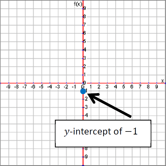
The y-intercept is -1, so we plot a point at -1 on the y-axis to begin.

Step 2 :

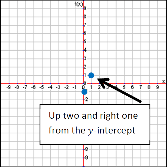
Next, the slope is 2 which means a rise of 2 and a run of 1. So we’ll move up two and right one to plot the next point.

Step 3 :

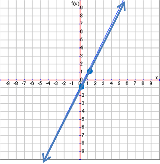
Finally, connect the dots with a line. This completes the graph of our linear function.

Example 2 :

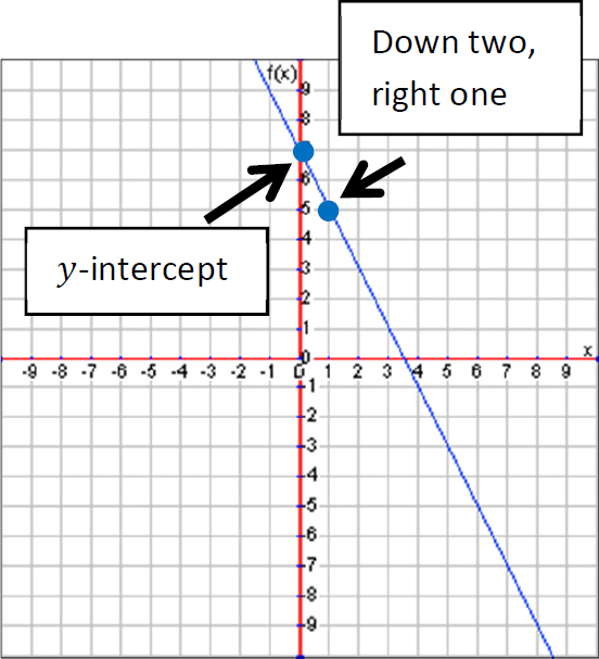
Graph : y = -2x + 7.

Solution :

Step 1 :

The y-intercept is 7, so we plot a point at 7 on the y-axis to begin.

Step 2 :

Next, the slope is -2 which means a rise of 2 and a run of 1. Since the slope is negative, we’ll move down two and right one to plot the next point.

Step 3 :

Finally, connect the dots with a line. This completes the graph of our linear function.

Example 3 :

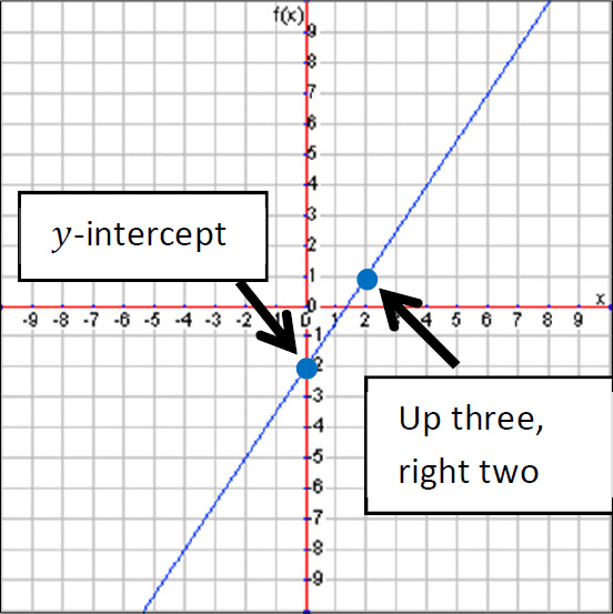
Graph : y = (3/2)x - 2.

Solution :

Step 1 :

The y-intercept is -2, so we plot a point at -2 on the y-axis to begin.

Step 2 :

Next, the slope is 3/2 which means a rise of 3 and a run of 2. So we’ll move up three and right two to plot the next point.

Step 3 :

Finally, connect the dots with a line. This completes the graph of our linear function.

Example 4 :

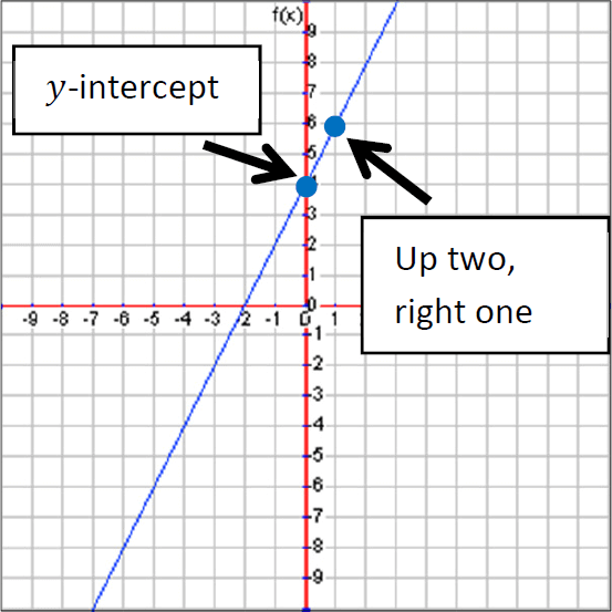
Graph : y = 2x + 2.

Solution :

Step 1 :

The y-intercept is 2, so we plot a point at 2 on the y-axis to begin.

Step 2 :

Next, the slope is 2 which means a rise of 2 and a run of 1. So we’ll move up two and right one to plot the next point.

Step 3 :

Finally, connect the dots with a line. This completes the graph of our linear function.

Kindly mail your feedback to v4formath@gmail.com

We always appreciate your feedback.